Chapter 8Neural Network Fundamentals
When rules run out
The methods of Chapter 7 never had to learn anything, because they counted, reweighted and factored, and every step was a fixed recipe applied to data. Many problems yield to that style and many do not.
Nobody can write down the rules that tell a photograph of a cat from one of a dog, or the rules that map an acoustic waveform to the sentence it encodes, or, to stay in this book, the rules that decide whether a film review is favourable. The knowledge is real but tacit, since we recognise the cat without being able to say what makes it one.
For such problems the way forward is to learn the mapping from examples, because the rule writing of Chapter 1 has nothing to write down. Show the machine thousands of labelled cases and let it adjust itself until it gets them right, in the hope that it captured the pattern rather than memorising the cases.
This chapter builds the machine that does the adjusting, and every model in the rest of this book is this machine enlarged, from the word2vec of Chapter 9 to the transformers of Part IV.
The neuron
The atom of the machine is deliberately simple. A single artificial neuron takes an input vector , forms a weighted sum with learnable weights and a bias , then passes the result through a nonlinear activation function :
The weighted sum is called the pre-activation, and it is a linear function of the input.
The activation is what lets the neuron represent anything more interesting than a line, because without it stacking neurons would be pointless, a composition of linear maps being just another linear map. The choice of is therefore not cosmetic but the thing that lets a network bend and curve and carve up its input space.
Activation functions
The historical first choice was a hard threshold, outputting if and otherwise. It captures the all or nothing firing of a real neuron and it is also useless for learning, because its derivative is zero everywhere it is defined and so gives no signal about which way to nudge the weights. Learning by gradients demands a smooth activation.
The sigmoid was the classic smooth replacement, , which squashes any real number into and is convenient when the output should read as a probability. Three values are worth knowing: , and .
It has two defects, and this book has already felt both. Its outputs are not centred on zero, which slows learning, and more seriously it saturates, since for large the curve flattens and its derivative approaches zero.
That derivative is , whose maximum sits at and is only , so even at its best a sigmoid shrinks the gradient passing through it by a factor of four. Stack that across many layers and you have the vanishing gradient that crippled the recurrent networks of Chapter 12.
The tanh function fixes half the problem, being zero centred over with a derivative at the origin of rather than . It preserves gradient better, which is why the recurrent networks of Chapter 12 and the gates of Chapter 13 used it.
The modern default fixes the other half. The rectified linear unit is , whose derivative for positive inputs is exactly , so it does not saturate on that side at all, and it is trivially cheap to compute. It has its own flaw, since a neuron stuck at has zero gradient and can die, which leaky variants patch by allowing a small negative slope.
The through line is the same for all of them. An activation must be nonlinear enough to give the network expressive power and smooth enough to give learning a gradient to follow.
The perceptron and its limit
Before layers, meet a single neuron on its own, because what it can and cannot do is the reason every network after it has a middle.
The perceptron is Equation (8.1) with a hard threshold. Frank Rosenblatt built one in 1958, in hardware, with motors adjusting potentiometers for weights, and it takes inputs, weights them, adds a bias, then fires if the total clears zero.
It also learns, by a rule so simple you can run it in your head. Show it an example, and if it is right change nothing, while if it is wrong nudge every weight in the direction that would have helped:
Rosenblatt proved this converges provided a solution exists, and that proviso is the whole story of this section.
What one neuron can do
A perceptron computes , which is the equation of a line in two dimensions, a plane in three and a hyperplane in general, so a perceptron draws one straight boundary and answers according to which side you fall on.
Plenty of useful functions are that shape, and here are two of them with weights you can check by hand.
| output for | |||||
| function | weights | ||||
| AND | 0 | 0 | 0 | 1 | , |
| OR | 0 | 1 | 1 | 1 | , |
AND at gives , so it fires, while at it gives and does not. That is one line, drawn between the single corner where both inputs are on and the three where they are not.
This is why perceptrons were exciting, because character recognition, simple sensor decisions and any judgement where the classes fall on opposite sides of a boundary all became learnable from examples rather than programmed.
Where it fails: XOR
Now try exclusive or, which fires when exactly one input is on.
| XOR | ||
|---|---|---|
| 0 | 0 | 0 |
| 0 | 1 | 1 |
| 1 | 0 | 1 |
| 1 | 1 | 0 |
Draw the four points and the trouble is visible. The two that should fire, and , sit on one diagonal, while the two that should not, and , sit on the other, so they interleave.
No single straight line separates one diagonal from the other, and the failure is not a lack of cleverness, since it can be proved in four lines. Suppose some computes XOR. Then:
| input | requirement | because XOR is |
|---|---|---|
| 0 | ||
| 1 | ||
| 1 | ||
| 0 |
Add the second and third requirements to get , then rearrange to . The first requirement says , so , and therefore , which contradicts the fourth requirement. No such weights exist.
Minsky and Papert published this in 1969 and the field’s funding and enthusiasm collapsed for a decade. The result is correct, while the conclusion drawn from it was not, because the fix was already known in principle: add a layer.
The fix: remap the input
Here is the network, with two hidden units using ReLU and then one output unit. All weights are small integers, so you can verify every number.
Run all four inputs through it.
| input | XOR | correct? | ||||||
| 0 | 0 | 0 | 0 | 0 | 0 | yes | ||
| 0 | 1 | 1 | 1 | 0 | 1 | yes | ||
| 1 | 0 | 1 | 1 | 0 | 1 | yes | ||
| 1 | 1 | 0 | 2 | 1 | 0 | yes | ||
It works, but how it works is the lesson, and that becomes visible if you throw away the input columns and look only at where each point landed.
| input in space | lands at | target |
|---|---|---|
| 0 | ||
| and | 1 | |
| 0 |
That table is the whole idea of deep learning. Four input points became three hidden points, because the two inputs that share a target, and , were mapped onto the same place, the hidden layer having decided they were the same kind of thing.
And now the problem is linear. In hidden space the target-1 point sits at , between the two target-0 points at and , and the output unit computes , which scores them , and , so one threshold at separates them cleanly.
The output unit is still just a perceptron and still draws one straight line. What changed is the space it draws that line in.
Why the remap is the whole idea
A hidden layer does not classify. It moves the data to a place where classifying is easy.
The last layer of almost every network in this book is a linear map followed by a softmax, which is a perceptron with more outputs and was never made cleverer. Everything before it exists to hand it a representation where a straight line will do, and once you see that, the rest of the book is one idea in many costumes.
| model | what it remaps, and into what |
|---|---|
| Multilayer perceptron | a fixed input vector, into a space where classes separate |
| Word embeddings (Ch. 9) | one-hot words, into a space where similar words sit close |
| Recurrent network (Ch. 12) | a sequence, into a hidden state carrying its history |
| Transformer (Ch. 16) | each token, into a vector shaped by the tokens around it |
Every row is the XOR trick at a different scale. Chapter 6 made the same complaint about one-hot vectors, that every word is equidistant from every other, and the answer there was a better space too.
The word for what a hidden layer produces is a representation, and learning good representations is what the field means when it says deep learning. XOR is the smallest example where you can watch it happen and check every number by hand.
The same trick on words
XOR is arithmetic, and words are the reason we are here, but the move is the same one and on a small enough vocabulary every number is still checkable by hand. Here is the whole corpus, in eleven short sentences.
| feed the cat | the cat sleeps | |
| feed the dog | the dog sleeps | |
| feed the horse | the horse sleeps | ride the horse |
| drive the car | park the car | |
| drive the bus | ride the bus |
That is five words and five things said about them, so tally which word appears with which context and the corpus becomes a grid.
| feed | sleeps | ride | drive | park | |
|---|---|---|---|---|---|
| cat | 1 | 1 | 0 | 0 | 0 |
| dog | 1 | 1 | 0 | 0 | 0 |
| horse | 1 | 1 | 1 | 0 | 0 |
| car | 0 | 0 | 0 | 1 | 1 |
| bus | 0 | 0 | 1 | 1 | 0 |
That grid is everything the model will ever be told, with no dictionary, no labels, and nobody anywhere saying that a cat is an animal.
The input space knows nothing
Feed a word to a network and it must arrive as numbers, and the obvious encoding gives each word its own dimension.
| word | one-hot input |
|---|---|
| cat | |
| dog | |
| horse | |
| car | |
| bus |
Five words, five dimensions. Now measure the ten pairs.
| pair | distance | cosine |
|---|---|---|
| cat, dog | 0 | |
| cat, horse | 0 | |
| cat, car | 0 | |
| cat, bus | 0 | |
| and the six remaining pairs, all identical | ||
Ten pairs and one distance, so cat is exactly as far from dog as it is from bus. This is the complaint of Chapter 6 with numbers attached.
One note before the fix, because the trouble with one-hot inputs is not the trouble XOR had. A single unit over five one-hot inputs carries five free weights, one per word, so it can fire for any subset you like and separability is not the problem. The problem is that every weight is private to a word, so nothing the model learns about cat can ever reach dog.
The fix: two hidden units
Insert a hidden layer of two units between the word and the answer. Its weights form a matrix , one row per word.
There is one output unit per context and each fires when its score is positive. Here are the weights, small integers again, so nothing is hidden in the arithmetic.
| hidden weights | output units | |||||
| word | row 1 | row 2 | context | |||
| cat | 2 | 0 | feed | 1 | ||
| dog | 2 | 0 | sleeps | 1 | ||
| horse | 2 | 1 | ride | 1 | 1 | |
| car | 0 | 2 | drive | 1 | ||
| bus | 1 | 2 | park | 1 | ||
The first step costs nothing, because a one-hot vector times simply selects a row of , so the multiplication is a lookup and the row it returns is the word’s embedding.
| word | ||
|---|---|---|
| cat | ||
| dog | ||
| horse | ||
| car | ||
| bus |
Now score every context for every word, where each cell is one multiplication and one addition. Bus sits at , so its ride score is and its park score is .
| word | feed | sleeps | ride | drive | park | fires for |
|---|---|---|---|---|---|---|
| cat | feed, sleeps | |||||
| dog | feed, sleeps | |||||
| horse | feed, sleeps, ride | |||||
| car | drive, park | |||||
| bus | ride, drive |
Read the last column against the corpus grid and every cell agrees, so eleven sentences are reproduced by ten numbers in and fifteen in the output layer.
Where the words landed
As with XOR, the lesson is where the points went, so throw away the score columns, keep the arrival, and group the words by the place they arrived at.
| lands at | arrived from | fires for |
|---|---|---|
| cat and dog | feed, sleeps | |
| horse | feed, sleeps, ride | |
| car | drive, park | |
| bus | ride, drive |
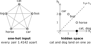
That is the XOR table again with words in it. Five input vectors became four hidden points, and two vectors that are orthogonal in the input, cat and dog, were mapped onto the same place because the corpus uses them identically. The hidden layer decided they were the same kind of thing, and the two tables say one thing at two scales.
| XOR | words | |
|---|---|---|
| input vectors | 4 corners of a square | 5 one-hot vectors |
| distances between them | 1 or | , every pair |
| hidden points | 3 | 4 |
| which two coincide | and | cat and dog |
| because they share | a target | every context |
Even XOR’s input space has some structure to work with, since two of its corners are closer than the other two, whereas one-hot inputs do not have that much. Every pair is apart, so every part of the arrangement in the table above was built by the hidden layer out of the corpus alone.
The other three did not collapse, and their spacing is the interesting part, so measure the pairs again in the hidden space. Dog repeats cat exactly, so its rows are left out.
| pair | input distance | hidden distance | hidden cosine | moved |
|---|---|---|---|---|
| cat, dog | 1.4142 | 0.0000 | 1.00 | together |
| cat, horse | 1.4142 | 1.0000 | 0.89 | together |
| car, bus | 1.4142 | 1.0000 | 0.89 | together |
| horse, bus | 1.4142 | 1.4142 | 0.80 | stayed |
| cat, bus | 1.4142 | 2.2361 | 0.45 | apart |
| horse, car | 1.4142 | 2.2361 | 0.45 | apart |
| cat, car | 1.4142 | 2.8284 | 0.00 | apart |
One distance became several. Horse sits between the animals and the vehicles because the corpus both rides it and feeds it, and bus sits between car and horse for the same reason. Nobody put them there, and they landed where their contexts sent them.
Nobody has to choose the numbers
Those weights were written down rather than learned, so that the arithmetic stays checkable, whereas training finds its own. Run gradient descent on the same eleven sentences with two hidden units and one output unit per context, then read the arrivals exactly as before.
| lands at | arrived from | fires for |
|---|---|---|
| cat and dog | feed, sleeps | |
| horse | feed, sleeps, ride | |
| car | drive, park | |
| bus | ride, drive |
Four groups again, and the same fires-for column, while the one-hot vectors on the left are the same five vectors, still apart and still carrying nothing.
Only the coordinates differ, and there is no reason they should not, since nothing in the loss fixes which direction is which and an axis on its own means nothing. Read the distances instead, which no rotation can change.
| pair | learned distance | hand-set distance |
|---|---|---|
| cat, dog | 0.0000 | 0.0000 |
| cat, horse | 1.9065 | 1.0000 |
| car, bus | 2.6205 | 1.0000 |
| horse, bus | 2.7856 | 1.4142 |
| cat, car | 3.3511 | 2.8284 |
Cat and dog arrive at the same point, identical to every digit, from five different random starts. The four nearest pairs come out in the same order as the hand-set ones, and after that the two orderings part company. Cat and car is the fifth nearest pair once the vectors are learned, where the hand-set space makes it the furthest of all seven. That costs nothing, since by then the words are unrelated anyway, but it is worth knowing that only the near end of such a ranking is stable.
What the remap buys
Collapsing cat onto dog is how a model answers a question it was never asked.
Delete one cell from the grid, so that the corpus never says feed the dog and dog now appears in one sentence only, the dog sleeps. Train both models on what is left, then ask each of them whether a dog can be fed.
| model | reading | |
|---|---|---|
| one-hot lookup, no hidden layer | 0.50 | a coin toss |
| two hidden units | 0.92 | yes |
The reason is in the weights. The lookup keeps one weight per word per context, so deleting the cell leaves that weight with no gradient and it never moves, which makes the answer whatever the bias happened to be. The model has nothing to say.
The network with a hidden layer has no weight for that cell at all, because it has a place for dog instead. Four facts survive the deletion, namely that the dog sleeps and that it is never ridden, driven or parked, and one corner of the plane satisfies all four. That corner already holds cat and horse, the feed unit covers it, so feed comes back for free.
That is what a word embedding is, and every model in Chapter 9 is this network grown larger, with a bigger vocabulary, a bigger hidden layer and a real corpus. Word2vec uses three hundred hidden units instead of two and millions of sentences instead of eleven, and the mechanism on this page does not change.
Try it yourself.
code/worked_examples/xor_to_words.pyprints every table above.--trainlearns the embedding instead of setting it, and--holdoutruns the deleted cell experiment. Change one sentence in the corpus, then watch which pair of words stops collapsing.
Layers, loss, and cost
A single neuron is a weak learner, and the power comes from arranging many into layers and stacking the layers so that each layer’s activations feed the next.
Such a network is called feed-forward, or a multilayer perceptron, and it applies an affine map and a nonlinearity at every layer. With enough hidden units it can approximate almost any function, which is what makes it a universal tool.
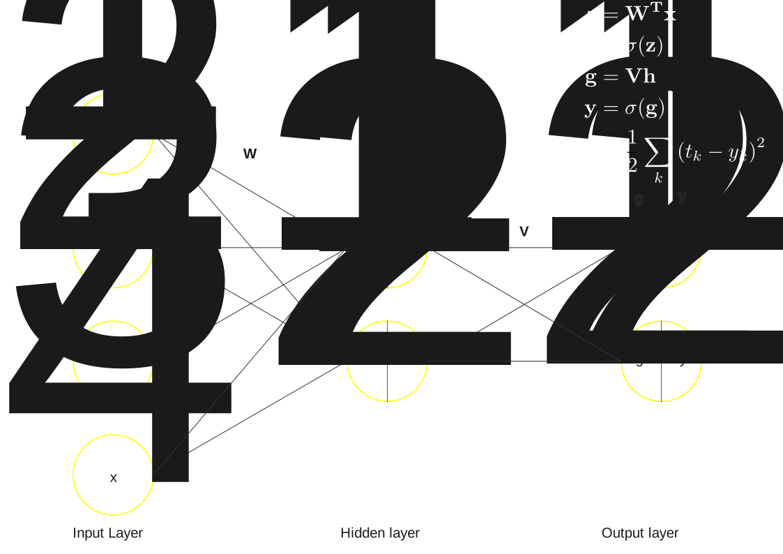
You have already met one such network, since the lookup, mix and softmax stack of the neural language model in Chapter 11 is exactly this, and so at bottom is every architecture that follows it.
To train a network we need a number saying how wrong it currently is. For a single training example the loss compares the prediction with the true target . For classification we do not have to invent one, because maximum likelihood produces it as soon as is read as a probability.
A binary target has two outcomes, so describes a Bernoulli draw:
The exponents do the selecting. At the second factor is one and the probability is , and at the first factor is one and it is . One expression therefore covers both outcomes.
Training wants the parameters that make the observed most likely, so take logs of Equation (8.4) and the product becomes a sum:
Now negate it, for two reasons. A log likelihood is highest when the model fits best, and gradient descent only moves downhill, so we need a quantity to minimise. Negation is strictly decreasing, so it leaves the best parameters where they are and turns that maximum into a minimum. It also fixes the scale, because a probability is at most , so its log is at most and the negative never falls below zero.
Negating Equation (8.5) is the whole step, and what it leaves is the cross-entropy loss:
So Equation (8.6) is the negative log likelihood of a single Bernoulli observation, and nothing about it was chosen for convenience.
It behaves exactly as a good loss should, so take the truth to be .
| prediction | loss | reading |
|---|---|---|
| nearly right, small penalty | ||
| hedging, moderate penalty | ||
| confidently wrong, severe penalty |
Cross-entropy rewards confident correctness and punishes confident error, which is the same pressure we met in the perplexity of Chapter 10, and that is no coincidence, because perplexity is the exponentiated cross-entropy of a language model.
Chapter 11 runs the same argument over outcomes, which is the form every later classifier in this book uses.
The loss is defined for one example, whereas what we actually minimise is the cost, the average loss over the whole training set seen as a function of all the parameters :
Learning is now a concrete goal: find the that makes as small as possible.
Gradient descent and backpropagation
We minimise the way you descend a hill in fog, by feeling which way is steepest downhill and then stepping that way. The direction of steepest increase is the gradient , so we step the opposite way:
where the learning rate sets the step size, so that too small a value makes training crawl while too large a value overshoots and diverges. Repeat this for many steps, in practice on small random batches of examples, and gradient descent walks the parameters downhill towards a good fit.
Equation (8.8) needs one thing, which is the gradient, meaning the partial derivative of the cost with respect to every weight, often millions of them. Computing those efficiently is the job of backpropagation, and it is nothing more exotic than the chain rule of calculus applied to the network’s layered structure. The error at the output travels backwards layer by layer, and each layer multiplies the gradient arriving from above by its own local derivative.
One result is worth carrying away because it recurs throughout the book. Pair a sigmoid or softmax output with the cross-entropy loss and the gradient of the loss with respect to the pre-activation collapses to
the prediction minus the target.
A nearly correct neuron, against , gets a gentle push of , while a confidently wrong one, against , gets a hard shove of .
This prediction minus target signal drove the neural language model of Chapter 11 and the classifiers of Chapter 14, and it is why cross-entropy and the sigmoid or softmax are always found together.
One training step, all the way through
Nothing makes this concrete like doing it once with numbers, so here is a tiny network with two inputs, two hidden ReLU units and one sigmoid output. The parameters start at these values:
| layer | weights | bias |
|---|---|---|
| hidden unit 1 | , | |
| hidden unit 2 | , | |
| output | , |
The training example is with target , and the learning rate is .
Step 1: forward.
Push the input through one layer at a time.
| quantity | arithmetic | value |
|---|---|---|
The network is barely better than a coin flip, which is what an untrained network should look like.
Step 2: backward.
Start at the output and use Equation (8.9), working back towards the input.
| gradient | arithmetic | value |
|---|---|---|
| , ReLU is open | ||
| , ReLU is open | ||
The ReLU derivative is a gate. Both units have , so both gates are open and multiply by , whereas had either been negative its gate would multiply by and every weight below it would get no signal at all on this example.
The signs differ because and have opposite signs, so hidden unit 1 pushed the output up and gets rewarded while hidden unit 2 pushed it down and gets corrected.
Step 3: update.
Apply Equation (8.8) to every parameter, biases included, since a bias is a weight on a constant input. A negative gradient makes the parameter go up.
| parameter | old | gradient | new |
|---|---|---|---|
The last two rows earn their place. Both gradients are exactly zero because and on this example, so a weight on an input that is off receives no signal and cannot move. The three biases do move, and leaving them out would give the wrong answer below.
Step 4: check it worked.
Run the same example forward again with all nine parameters at their new values.
| before | after | ||
|---|---|---|---|
| gate now shut | |||
The prediction moved towards the target and the loss fell by nearly two thirds. That is the whole algorithm, and everything after this chapter is the same four steps run on larger networks, over more examples, many millions of times.
One step was large enough to change the network’s shape, which is worth noticing. Hidden unit 2 was pushing the output down, so the update drove negative, and the unit’s gate is now shut on this input. It contributes nothing to the next forward pass and will receive no gradient from this example again. That is the dying ReLU of Section 8.2.1 arriving in a worked example rather than as a warning, and a learning rate of is what made one step big enough to cause it.
Generalisation: the whole point
Given enough capacity, a network trained by Equation (8.8) will drive its training cost towards zero, and that is not the goal. Mistaking it for the goal is the central hazard of the field.
The goal is generalisation, meaning low error on data the model has never seen. A model that merely memorised its training examples would score perfectly on the training set and uselessly on anything new, which is overfitting, fitting the noise and idiosyncrasy of the training sample instead of the pattern that also governs future data.
We detect it with the discipline the whole field lives by, which Chapter 14 makes concrete: hold out a test set the model never trains on, and judge the model only by its error there.
Everything that combats overfitting serves that one end, whether regularisation, early stopping, dropout or, above all, more data. A neural network is valuable exactly to the extent that what it learned transfers beyond its training data.
One machine, many chapters
That is the entire apparatus: a neuron, a nonlinearity, a loss averaged into a cost, gradient descent to minimise it, backpropagation to supply the gradients, and a test set to keep the whole enterprise honest.
Nothing in the chapters ahead adds a new principle to that list, because what they add is architecture, meaning particular wirings of neurons suited to particular data.
The first use is immediate. Turn this machine loose on the distributional hypothesis of Chapter 6 by training vectors to predict their contexts, and out come the word embeddings of Chapter 9. That is the same dense geometry the counting of Chapter 7 produced, now trained rather than computed, and from there the story is one of ever cleverer architectures, recurrent, gated and attentional, built from these identical parts.
Further reading.
Rumelhart et al. (1986) made backpropagation and gradient trained
multilayer networks widely known. For activations, loss functions,
optimisation and regularisation in full depth, go to Goodfellow et al.
(2016). Goldberg (2015) covers the same ground as a primer written for
natural language processing. On how initialisation and momentum shape
the optimisation this chapter only sketches, see Sutskever et al.
(2013). Every gradient in the worked step above is what
torch.autograd computes on your behalf, and the four steps
of this section are what the two lines loss.backward() and
optimizer.step() stand for in any modern training loop.
The sigmoid and its shrinking gradient. Compute , and . Then use to find the at which the derivative is largest, and state that maximum. In one sentence, relate the number to the vanishing gradient of Chapter 12.
What cross-entropy rewards. For a true label , evaluate Equation (8.6) at , and . Do the three numbers behave as a good loss should? Repeat for and confirm the symmetry.
Prediction minus target. Use Equation (8.9). Give for a neuron predicting when the truth is , and for one predicting when the truth is . Which gets the larger update? Why is that the behaviour you want?
Redo the worked step with a shut gate. Repeat the four step worked example, changing only from to . Show that is now negative, so and the ReLU gate is shut. Which gradients become zero? Which parameters do not move at all on this example, and why?
One gradient step. A single weight has value and . Apply Equation (8.8) with and report the new . What happens to training if is set to instead?
Fitting is not the goal. A network reaches error on its training set and on held out data. Name the phenomenon. Explain what went wrong, in terms of pattern against memorisation. List two things you could change to improve the held out number. Why is the test set the only honest judge?
Let autograd check your arithmetic. Build this
chapter’s network in torch, two inputs, two hidden ReLU
units and one sigmoid output, starting from the same weights and biases
and using the same
with
.
Call backward() and compare what it reports against the
Step 2 table, then apply one step at
and confirm that
reaches
and
falls to
.
Now print the pre-activation of hidden unit 2 and say what has happened
to that unit, and which sentence of this chapter predicted it.
Code for this chapter
Each one reproduces the tables above. Open it in Colab, change an input and watch which numbers move.
-
xor_to_words.pyThe XOR remap, done on wordsFive words, five contexts, two hidden units. Cat and dog land on the same point, and a deleted fact comes back.
standard library only Run it in Colab Notebook Source
From Natural Language Processing: From Corpus Statistics to Grounded LLMs, by Ramaseshan Ramachandran.