Chapter 13Gated Recurrence: LSTM and GRU

Addition instead of multiplication

Chapter 12 left the recurrent network with a precise complaint, not a vague one.

Equation (12.5) showed that a gradient travelling back through time is multiplied by one Jacobian per step. Each Jacobian is $\operatorname{diag}(\tanh')\,U$, so the product behaves like a number raised to the power of the distance.

Below one it vanishes. Above one it explodes. Nothing holds it at one.

The diagnosis contains the cure. If repeated multiplication is what destroys the gradient, then give the state a path that does not multiply.

A gated network does exactly that. It keeps a memory that is updated by addition, and it learns how much of the old memory to carry forward.

The LSTM cell

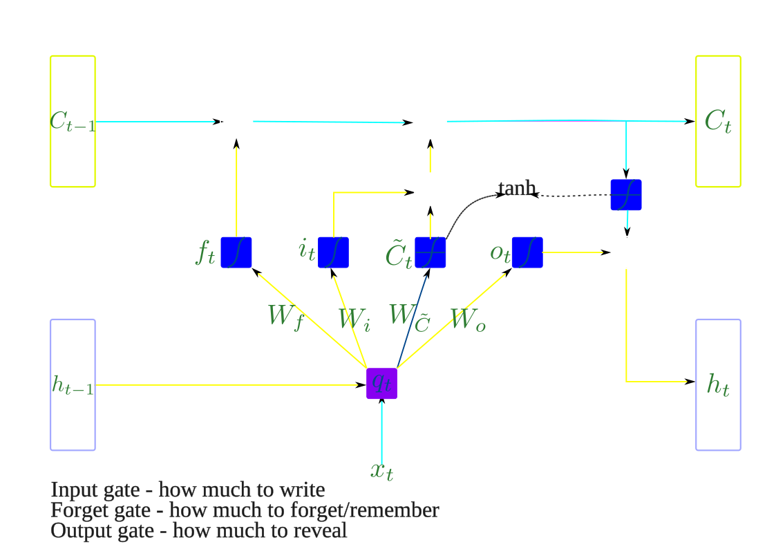
The long short-term memory network carries two vectors rather than one.

The cell state $C_t$ is the memory. The hidden state $h_t$ is what the rest of the network sees.

Three gates control the traffic. Each is a sigmoid layer reading the same input, the previous hidden state concatenated with the current word, so each produces numbers between $0$ and $1$.

$$\begin{align} f_t &= \sigma\!\big(W_f\,[h_{t-1}, x_t] + b_f\big) && \text{(forget gate)}, \label{eq:lstm-f}\\ i_t &= \sigma\!\big(W_i\,[h_{t-1}, x_t] + b_i\big) && \text{(input gate)}, \label{eq:lstm-i}\\ o_t &= \sigma\!\big(W_o\,[h_{t-1}, x_t] + b_o\big) && \text{(output gate)}, \label{eq:lstm-o}\\ \tilde{C}_t &= \tanh\!\big(W_C\,[h_{t-1}, x_t] + b_C\big) && \text{(candidate)}. \label{eq:lstm-cand} \end{align}$$

A gate value of $0$ closes the channel completely. A value of $1$ opens it. Everything in between is a partial opening, which is what makes the whole thing differentiable.

The cell state is then updated in one line, and that line is the reason the architecture exists:

$$\begin{equation} C_t \;=\; f_t \odot C_{t-1} \;+\; i_t \odot \tilde{C}_t . \label{eq:lstm-cell} \quad\text{(13.1)} \end{equation}$$

Read it as two decisions. The forget gate says what fraction of the old memory survives. The input gate says how much of the new candidate to admit.

The hidden state is a filtered view of that memory:

$$\begin{equation} h_t \;=\; o_t \odot \tanh(C_t). \label{eq:lstm-h} \quad\text{(13.2)} \end{equation}$$

So the network can hold something in $C_t$ for many steps without exposing it, and reveal it only when the output gate opens.

Why this fixes the gradient

Differentiate Equation (13.1) along the cell state path. The result is startlingly simple:

$$\begin{equation} \frac{\partial E}{\partial C_{t-1}} \;=\; f_t \odot \frac{\partial E}{\partial C_t}. \label{eq:lstm-grad} \quad\text{(13.3)} \end{equation}$$

No weight matrix. No $\tanh$ derivative. The gradient is multiplied by the forget gate and nothing else.

Compare the two routes directly.

At $f = 0.99$ a gradient still carries one per cent of its strength after $500$ steps. At $0.5$ it is gone before step $50$.

Be careful about what has changed. The LSTM did not remove the decay. It put the decay rate under the network’s control.

That is enough, and it is the whole contribution. $f_t$ is learned, so the network can decide to keep a memory alive when the task rewards it. $\operatorname{diag}(\tanh')\,U$ was never anybody’s decision.

The bias that decides everything

Here is a detail the lectures single out, and it is worth a section because skipping it is so common.

At the start of training the weights are small and random, so Equation (13.4) gives $f_t \approx \sigma(b_f)$.

The default initialisation sets $b_f = 0$. That makes $f_t \approx 0.5$.

Look at the first row against the previous table. A default-initialised LSTM decays at exactly the rate the plain RNN did.

So it starts out no better than the architecture it was invented to replace, and it has to climb out of that by learning.

Set $b_f = 2$ instead, as recommend, and $f_t$ begins at $0.8808$. After $47$ steps the gradient retains $2.57 \times 10^{-3}$ rather than $7.11 \times 10^{-15}$.

That is $3.6 \times 10^{11}$ times more signal, from changing one number before training starts.

The lesson generalises past LSTMs. A model that appears incapable of a task is sometimes a model whose initialisation put it somewhere it could not leave.

One cell, worked

Take a cell with two units and an input of size two, and set $b_f = 1$.

$$h_{t-1} = (0.10,\, -0.20), \qquad C_{t-1} = (0.50,\, 0.30), \qquad x_t = (0.60,\, 0.40).$$

Every gate reads the same concatenated vector:

$$q \;=\; [h_{t-1}, x_t] \;=\; (0.10,\, -0.20,\, 0.60,\, 0.40).$$

Split the cell update into its two terms and the arithmetic becomes plain.

The forget gate sits at $0.80$ and $0.70$, so most of the old memory survives the very first step. That is the $b_f = 1$ initialisation already doing its job.

And notice how $C_t$ was reached. By addition, not by a matrix multiplication. That single structural fact is the difference from Equation (12.8), and it is why Equation (13.3) looks the way it does.

The GRU: the same trick, fewer parts

The gated recurrent unit asks whether four gates were ever necessary.

It keeps one state vector instead of two, and two gates instead of three.

$$\begin{align} z_t &= \sigma\!\big(W_z\,[h_{t-1}, x_t] + b_z\big) && \text{(update gate)}, \label{eq:gru-z}\\ r_t &= \sigma\!\big(W_r\,[h_{t-1}, x_t] + b_r\big) && \text{(reset gate)}, \label{eq:gru-r}\\ \tilde{h}_t &= \tanh\!\big(W\,[\,r_t \odot h_{t-1},\; x_t\,] + b\big), \label{eq:gru-cand}\\ h_t &= (1 - z_t) \odot h_{t-1} \;+\; z_t \odot \tilde{h}_t. \label{eq:gru-h} \end{align}$$

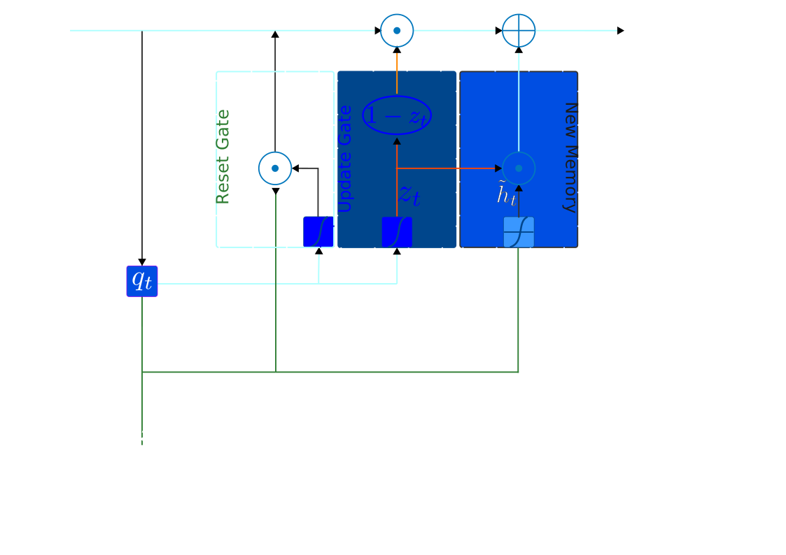
Equation (13.11) is the interesting line. The coefficients are $(1 - z_t)$ and $z_t$, so they sum to one.

The LSTM used two independent gates for those two jobs, and could in principle forget everything while adding nothing. The GRU ties them, so forgetting more means admitting more.

The reset gate does a different job. It decides how much of the old state the candidate may see, which lets the unit propose something genuinely new when the topic changes.

Running the same numbers as above through a GRU gives this.

What a gate costs

Each gate reads a vector of length $H + d$ and produces $H$ numbers, so it costs $H(H + d) + H$ parameters. Count the gates and you have the model.

Those figures use $d = 100$ and $H = 500$. A GRU is three quarters the size of an LSTM, which here is $300{,}500$ fewer parameters and a proportionally faster step.

On most tasks the two score within noise of each other . So the choice is usually made on size and speed rather than on quality, and the GRU often wins on those.

Try it yourself. code/worked_examples/gated.py produces every table in this chapter. --highway compares the two decay routes, --bias shows what $b_f$ does, --step runs the single cell through both architectures, and --params counts the gates.

Run it in ColabNotebookSource

The end of the recurrent road

Gating worked. From roughly 2014 to 2017 the LSTM was the default for almost every sequence task, and it powered the first generation of neural machine translation.

Two problems remained, and neither is about gradients.

The first is sequential computation. Equation (13.1) needs $C_{t-1}$ before it can compute $C_t$. So the time steps cannot be computed in parallel, however many processors are available.

That is a hard ceiling on training speed, and it arrived exactly when hardware was becoming massively parallel.

The second is the bottleneck. Everything the model knows about the prefix has to fit in one fixed-size vector.

Gating made that vector’s contents last longer. It did not make the vector bigger, and a whole paragraph still has to be squeezed into it.

Both problems have the same shape. They come from insisting that information travel through the sequence, one step at a time.

The next idea removes that insistence. Let every position look directly at every other position, with no intervening steps. Distance stops mattering, and the computation parallelises because nothing waits for anything.

That is attention, and it is the subject of Chapter 16.

Before that, one chapter closes Part III on a different note. Everything from Chapter 10 to here has built models. None of it has said how you would know whether one is any good.

Chapter 14 answers that. It takes the simplest task these models are put to, and uses it to establish the evaluation discipline the rest of the book depends on.

Further reading.

is the original LSTM paper. introduce the forget gate and the bias initialisation of Section 1.3. propose the GRU. search thousands of gated architectures and find no consistent winner, which is the best evidence that the gating idea matters more than its packaging. is the clearest diagram-led explanation of the LSTM in existence and worth reading alongside this chapter.