Chapter 10n-gram Language Models and Perplexity

Guess the next word

Finish this sentence.

You said are. Everyone says are. Now try this one.

Here the answers spread out. Is, does, time, longer are all reasonable. You did not pick one answer. You held several, ranked.

That ranking is the subject of Part III. A model that can produce it is a language model. The rest of this book is a series of steadily more capable ways to build one.

What you used to answer

Notice how much you brought to a two word prompt.

Lexical knowledge told you which words exist and which are common. Syntactic rules told you that How are needs a subject next. Semantic cues ruled out How are cement. World knowledge told you that people greet each other this way. Pragmatics told you the sentence was a greeting rather than a question about health.

Five kinds of knowledge, none of them written down anywhere, all applied in under a second.

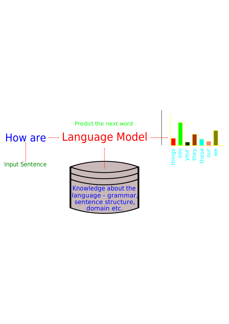
The engineering question is how to put that box on a computer. For thirty years the field tried to write the five knowledge sources down as rules. It did not work, for the reasons Chapter 1 gave.

This chapter takes the other road. Do not encode the knowledge. Count how often things happened, and let the counts stand in for all five.

That sounds far too crude to work. It works very well. Where it fails, it fails in ways that point straight at what comes next.

What a language model is

A language model assigns a probability to a sequence of words. That is the whole definition.

Pause on how strange it is. Nothing in it mentions grammar, meaning, or truth. A language model is a probability distribution over strings.

Yet this one idea is the foundation of everything after. The neural models of Chapter 11, the recurrent networks of Chapter 12, and the large language models of Chapter 17 all answer the same question. Given what has been said so far, what comes next, and with what probability? Only the machinery changes.

Why anyone wants one

Historically, because many language technologies reduce to choosing between candidate word sequences.

A speech recogniser hears a signal that fits both “recognise speech” and “wreck a nice beach”. It must pick one. A translation system generates a dozen candidate renderings and must rank them. A spelling corrector must decide whether “their going home” was meant to be “they’re going home”.

In every case the winning move is the same. Prefer the candidate the language model scores higher.

Today the motivation is more direct. A modern large language model is a language model in exactly this chapter’s sense. It produces its output one next word distribution at a time.

The chain rule

We want the joint probability of a sentence $W = w_1 w_2 \cdots w_n$. The chain rule of probability factorises it exactly, with no approximation:

$$\begin{equation} p(w_1 w_2 \cdots w_n) \;=\; \prod_{i=1}^{n} p\big(w_i \mid w_1, \ldots, w_{i-1}\big). \label{eq:chainrule} \quad\text{(10.1)} \end{equation}$$

Equation (10.1) converts one impossible problem into $n$ merely difficult ones. The impossible problem was a distribution over all sentences. The difficult one is a distribution over the next word, given a history.

It also shows why a language model is a generative model. Sample from the first factor, append the word, condition on it, and sample again. Repeat until you draw the stop symbol. You have written a sentence.

The difficulty that remains is the history. The context $w_1, \ldots, w_{i-1}$ can be arbitrarily long, and almost every particular history is one nobody has ever seen.

No corpus contains reliable statistics for the exact prefix “The results of the 2026 municipal elections in Tenkasi suggest”. It has appeared once, in this book.

The Markov assumption

The n-gram model’s answer is bold. Forget the past.

More precisely, assume the next word depends only on the previous $n-1$ words:

$$\begin{equation} p\big(w_i \mid w_1, \ldots, w_{i-1}\big) \;\approx\; p\big(w_i \mid w_{i-n+1}, \ldots, w_{i-1}\big). \label{eq:markov} \quad\text{(10.2)} \end{equation}$$

With $n = 2$, a bigram model, each word depends only on its predecessor. With $n = 3$, a trigram model, on the previous two. With $n = 1$, a unigram model, on nothing at all.

This is a Markov assumption, and it is plainly false. In “The book that the committee rejected was short” the verb agrees with book, eight words away.

The assumption is not made because it is true. It is made because it buys something we cannot otherwise have: contexts short enough to recur.

The history “of the” appears thousands of times in a modest corpus. Statistics conditioned on it are trustworthy. The history in the Tenkasi example appears once, and statistics conditioned on it are worthless.

So the whole art of n-gram modelling is one trade off. Longer context means a sharper prediction and thinner evidence. Shorter context means a blunter prediction and firmer evidence.

Estimating by counting

How do we get the conditional probabilities? By the most honest method available. Counting.

The maximum likelihood estimate of a bigram probability is the fraction of times the context was followed by the word in question:

$$\begin{equation} p_{\text{MLE}}\big(w \mid c\big) \;=\; \frac{\operatorname{count}(c, w)}{\operatorname{count}(c)}. \label{eq:mle} \quad\text{(10.3)} \end{equation}$$

That is all. No optimisation, no training loop. Read the corpus, keep two counters, divide.

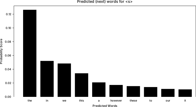
A corpus small enough to check

We will use three sentences for the whole chapter, so that every number can be verified by hand.

The word the occurs three times. Twice it is followed by cat, once by dog. So

$$p_{\text{MLE}}(\text{cat} \mid \text{the}) = \tfrac{2}{3}, \qquad p_{\text{MLE}}(\text{dog} \mid \text{the}) = \tfrac{1}{3},$$

and every other continuation of the has probability zero. Hold on to that zero. It becomes the villain of the chapter.

Conventions that change the numbers

Before any two implementations of Equation (10.3) can agree, three bookkeeping conventions must match. These sound like pedantry. Each one changes the answers, and Project 4 checks them exactly.

Padding.

Each sentence is padded with $n-1$ start symbols <s> and one stop symbol </s>.

The start padding gives the first real word a context, so a bigram model can speak of $p(\text{the} \mid \texttt{<s>})$.

The stop symbol does something deeper. It makes sentence length part of the model.

Without it the model only ever assigns mass to continuing, never to stopping. The probabilities of all sentences of all lengths then sum to more than one. With it, ending a sentence is an event like any other.

Unknown words.

A model trained on our three sentences will one day meet the word elephant.

The remedy is a designated symbol <unk>. Every word absent from the training vocabulary maps to it, and <unk> is an ordinary vocabulary item. So the vocabulary of our corpus is

$$V = \{\text{the, cat, dog, sat, ran}\} \cup \{\texttt{</s>}, \texttt{<unk>}\}, \qquad |V| = 7 .$$

Note what is not in $V$. The start symbol is context only. It is never predicted, so it never needs a probability, and it must never be mapped to <unk>.

What gets scored.

Probabilities, and later perplexity, are computed over the predicted tokens. That means the words of the sentence plus the one </s>. The start padding is never scored.

State these three and Equation (10.3) is reproducible to the last decimal. Omit them and two correct programs will disagree.

The zero problem and smoothing

Our model believes $p(\text{sat} \mid \text{dog}) = 1$ and $p(\text{ran} \mid \text{dog}) = 0$.

The first claim is merely overconfident. The second is fatal. Under the chain rule a single zero factor drives the whole sentence to probability zero, and its perplexity to infinity.

Yet “the dog ran” is perfectly good English. It just failed to appear in three sentences of training data. The model has confused unseen with impossible.

The remedy is to smooth. Shave a little mass off what we saw and hand it to what we did not. The simplest scheme is add-$\alpha$ smoothing, which pretends every vocabulary item was seen $\alpha$ extra times in every context:

$$\begin{equation} p_{\alpha}\big(w \mid c\big) \;=\; \frac{\operatorname{count}(c, w) + \alpha} {\operatorname{count}(c) + \alpha\,|V|}. \label{eq:addalpha} \quad\text{(10.4)} \end{equation}$$

The $\alpha|V|$ in the denominator is exactly what makes the probabilities sum to one again. That is why the vocabulary convention matters, and why </s> and <unk> have to be counted in $|V|$.

Watching the mass move

Set $\alpha = 1$ and $|V| = 7$, and look at every continuation of the. The context was seen $3$ times.

Both columns sum to one, as they must. The two seen words gave up $0.5$ between them, and the five unseen words received $0.1$ each.

The counts did not change. The belief did.

Now the same table for the context dog, which was seen only once.

This is the repair we wanted. $p(\text{ran} \mid \text{dog})$ has risen from $0$ to $0.125$, so “the dog ran” is no longer impossible.

It is also where add-$\alpha$ shows its weakness. Moving $p(\text{sat} \mid \text{dog})$ from $1.00$ to $0.25$ is not a shave. It is a scalping, and the evidence for it was a single observation.

The effect scales badly. With a realistic vocabulary of tens of thousands, the denominator is dominated by $\alpha|V|$. Nearly all the mass then goes to events nobody has ever seen.

So in practice one uses a small $\alpha$, tuned on held out data. Or one of the better schemes in Section 1.8.

The principle never changes. Every language model, up to the largest, must reserve belief for things it has not seen.

Perplexity: measuring a language model

Two colleagues each hand you a language model. Which is better?

The models are distributions, so let the data decide. The better model is the one that finds held out text less surprising. That is to say, it assigns the text higher probability.

Raw probabilities are unwieldy, because they shrink exponentially with length. So we normalise. The average negative log probability per predicted token is the model’s cross-entropy on the text:

$$\begin{equation} H(W) \;=\; -\frac{1}{N} \sum_{i=1}^{N} \log_2 p\big(w_i \mid \text{context}_i\big), \label{eq:crossent} \quad\text{(10.5)} \end{equation}$$

measured in bits per token. Its exponential is the perplexity:

$$\begin{equation} \operatorname{PP}(W) \;=\; 2^{\,H(W)} . \label{eq:ppl} \quad\text{(10.6)} \end{equation}$$

Here $N$ counts the predicted tokens. The words plus </s>, by the convention above.

Perplexity has a clean reading. It is the model’s effective branching factor, the size of the uniform distribution that would be equally surprised.

A perplexity of $100$ means the model is as uncertain at each step as if it were choosing among $100$ equally likely words. Lower is better. A model that knew the text by heart would score $1$.

And the zero we worried about gives $\log 0 = -\infty$, hence perplexity $\infty$. That is the formal statement of why unsmoothed models are unusable.

One perplexity, worked in full

Take the bigram model with $\alpha = 1$ and score the sentence the cat sat. Padded, it is <s> the cat sat </s>, so there are four predicted tokens.

Each row applies Equation (10.4) with $|V| = 7$.

The count column is $\operatorname{count}(c, w)$ and of is $\operatorname{count}(c)$. Every probability is $(\text{count} + 1) / (\text{of} + 7)$.

Now finish it:

$$H \;=\; -\frac{-6.8138}{4} \;=\; 1.7034 \text{ bits per token}, \qquad \operatorname{PP} \;=\; 2^{1.7034} \;=\; \mathbf{3.2568} .$$

So the model is about as unsure at each step as if it were choosing uniformly among $3.26$ words. The vocabulary holds $7$. On a corpus this small, that is a respectable score.

Two details in that table are worth naming. The first row scores the in the context <s>, which is why the padding exists. The last row scores </s>, which is why $N = 4$ and not $3$.

Choosing $\alpha$, and why the test set must be new

Perplexity gives us a way to pick $\alpha$. Try several and keep the best.

The catch is which text you measure on. Here are two sentences. The cat sat is in the training data. The dog ran is not, though every word of it is, and only the bigram $(\mathit{dog}, \mathit{ran})$ is new.

The two columns tell opposite stories.

The seen column falls all the way down. Less smoothing always looks better on text the model has memorised, and it would keep improving as $\alpha \to 0$.

The held out column is a U. It bottoms at $\alpha = 0.10$ and rises on both sides.

Both sides of that U have a cause. Too little smoothing and the single unseen bigram is crushed towards zero probability. Too much and the seen bigrams are robbed to pay for events that never happen.

Tuning on training text would have chosen $\alpha = 0.01$, which scores $4.3297$ on new text against the best available $3.2047$. That is $1.35$ times worse, from a decision that looked correct at the time.

Two cautions

Perplexity is only comparable across models that share a vocabulary and a tokenisation. A model with a smaller vocabulary has an easier problem, and the subword tokenisers of Chapter 5 change $N$ itself.

Perplexity also measures surprise, not usefulness. It correlates with downstream quality and does not guarantee it. Both cautions return with force in Chapter 21.

The curse of dimensionality

Everything so far suggests a simple way to improve the model. Use a longer context. If bigrams are good, trigrams should be better.

They are, for a while. Then the arithmetic stops you.

An n-gram model needs one number per history and word. There are $|V|^{n-1}$ possible histories, and within each one $|V| - 1$ free choices, since the last probability is fixed by the others:

$$\begin{equation} \text{parameters} \;\approx\; |V|^{\,n-1} \times (|V| - 1). \label{eq:ngram-params} \quad\text{(10.7)} \end{equation}$$

That exponent is the whole problem.

Take the bottom right cell. A 5-gram model over a $50{,}000$ word vocabulary has about $3.1 \times 10^{23}$ parameters.

Now count what could fill them. A corpus of a trillion tokens contains at most a trillion distinct 5-grams, one per position. So at most one cell in $3 \times 10^{11}$ can hold a nonzero count.

The counts do not merely get thin. Almost the entire table is empty. No corpus that will ever be assembled can change that.

Three consequences follow, and the lectures name them.

Data sparsity. Most n-grams have zero or tiny counts, so their probabilities cannot be estimated reliably.

Overfitting. The model latches onto the exact phrases in the training text and generalises to nothing else.

Computational cost. Storing and searching the table grows with the same exponent.

Beyond counting

The framework can be pushed further than add-$\alpha$, and three techniques matter.

Pruning discards n-grams with low counts. It saves space and removes estimates that were never trustworthy.

Interpolation mixes the orders. When the trigram evidence is thin, lean on the bigram. When the bigram fails too, lean on the unigram:

$$\begin{equation} p(w_3 \mid w_1, w_2) \;=\; \lambda_1\,p_1(w_3) \;+\; \lambda_2\,p_2(w_3 \mid w_2) \;+\; \lambda_3\,p_3(w_3 \mid w_1, w_2), \label{eq:interpolation} \quad\text{(10.8)} \end{equation}$$

subject to the one constraint $\lambda_1 + \lambda_2 + \lambda_3 = 1$. The weights say how much to trust each level of context, and they are tuned on held out data like any other hyperparameter.

Backoff does the same job with a switch rather than a blend. Use the trigram if you have seen it, otherwise drop an order and try again.

Interpolation, worked

Take a four sentence corpus, so that the trigram counts can run out while the bigram counts survive.

Set $\lambda_1 = 0.1$, $\lambda_2 = 0.3$ and $\lambda_3 = 0.6$, and take four queries in decreasing order of evidence. All three estimates below are unsmoothed, so the failures are visible.

Read the four rows as a staircase.

Row one has full evidence at every order. The trigram cat sat on was seen twice and never continued any other way. So all three estimates are high, and so is the mixture.

Row two shows what the extra context buys. The trigram is sharper than the bigram, $0.6667$ against $0.4286$, because on the narrows the field more than the alone.

Row three is the one that matters. The trigram on the cat never occurred, so $p_3 = 0$, and a pure trigram model would call the phrase impossible. The bigram has seen the cat twice and says $0.2857$. The mixture returns $0.0964$ and the sentence survives.

Row four is the last resort. The word ran never follows the anywhere in this corpus, so both higher orders fail. Only the unigram is left. The answer is small. What matters is that it is not zero.

Kneser-Ney smoothing is the state of the counting art, and it refines the lowest order term. What matters for an unseen context is not how often a word occurs but in how many distinct contexts it does. The word Francisco is common yet occurs almost only after San, so it deserves very little unseen-context mass. These refinements carried speech recognition and translation for two decades.

Try it yourself. code/worked_examples/ngram_lm.py produces every table in this chapter, using the same conventions the autograder enforces. --counts prints the two smoothing tables, --perplexity the four row calculation, --alpha the U shape, --params the parameter explosion, --interpolate the staircase, and --unk what happens to a word the model has never met.

Run it in ColabNotebookSource

What counting cannot fix

Smoothing repairs the zeros. Interpolation repairs thin evidence. Neither touches the two real blindnesses, and both are structural.

The first is the Markov assumption. The model cannot know that book, eight words back, governs the verb it is about to emit. Eight words back does not exist for it. Raising $n$ does not solve this, because the parameter table of Equation (10.7) explodes long before $n$ reaches eight.

The second is that words are opaque strings. Suppose the corpus contains the cat sat many times and the dog only once. A counter has no way to let cat lend statistical strength to dog, because to a counter they are two unrelated symbols.

Chapter 9 already built the cure for the second problem. Words became vectors, and similar words came out near each other. What was missing was a way to put those vectors to work on prediction.

That is exactly what the next chapter does. It keeps the task, the corpus, the smoothing instinct and the perplexity yardstick, and replaces the count table with a network.

Further reading.

cover this material with more smoothing variants and worked examples. remains the definitive empirical comparison of smoothing methods. treat the statistical foundations in depth. introduce the smoothing method that held the record for years. The class-based n-grams of are an early attempt to share statistical strength between related words, which is the problem Chapter 11 solves properly. is where the entropy of a text was first proposed as something measurable, and it is still worth reading.