Chapter 3The Empirical Laws of Text

Counting words, seriously

Before this book fits a single model, do something that sounds too simple to be scientific. Take a large body of text. Count how often each word occurs. Then stare at the counts.

This is the cheapest experiment in natural language processing. A few lines of shell script will do it. It also produces one of the most consequential findings in the field.

Language is wildly and lawfully unbalanced. Every system we build afterwards either respects that imbalance or is quietly broken by it.

Run the experiment on any sizeable English corpus and the same picture appears. A handful of words take a startling share of all running text. Words like the, of, and, to and a.

The Brown corpus makes a good witness, and this chapter measures it repeatedly. Every figure comes from autograder/nlp_pipeline.py. That is the tokeniser and fitting code Project 1 is graded against, so the numbers here are the ones your own submission should reproduce.

Under it Brown holds $1{,}023{,}734$ tokens and $44{,}324$ distinct words. The alone is $6.84$ per cent of all tokens. The ten most frequent words together are $24.1$ per cent.

A different tokeniser gives different totals. A stricter rule keeping only fully alphabetic tokens drops $V$ to $40{,}234$. Neither is wrong, and neither is comparable to the other. State the tokeniser whenever you state a count.

At the other end of the table something stranger shows up. Almost half of all distinct words occur exactly once. In Brown the figure is $39.5$ per cent, and $54.3$ per cent occur twice or fewer. These singletons have a name, hapax legomena, which is Greek for “said once”. That they are so abundant is the first sign that word frequency does not behave the way intuition expects.

Two clarifications before we go on, because the vocabulary of counting causes confusion. A token is a running occurrence of a word. A type is a distinct word. The sentence “the cat saw the dog” has five tokens but four types, because the occurs twice. Everything in this chapter is a statement about how types and tokens relate.

Zipf’s law

Order the types by frequency, most frequent first. Give each one a rank. The most frequent word has rank 1, the next has rank 2, and so on.

George Kingsley Zipf did this in the 1930s, by hand, in heroic quantity. He found that frequency and rank trade off almost exactly inversely:

$$\begin{equation} f(r) \;\approx\; \frac{C}{r^{\alpha}}, \qquad \alpha \approx 1, \label{eq:zipf} \quad\text{(3.1)} \end{equation}$$

where $f(r)$ is the frequency of the rank-$r$ word and $C$ is a constant of the corpus.

Literally, the second word is about half as frequent as the first. The tenth is about a tenth as frequent. The hundredth is about a hundredth.

A power law is a straight line

Take logarithms of both sides. Equation (3.1) becomes

$$\begin{equation} \log f(r) \;=\; \log C \;-\; \alpha \log r, \label{eq:zipf-log} \quad\text{(3.2)} \end{equation}$$

which is $y = mx + c$ with $y = \log f$, $x = \log r$, slope $m = -\alpha$ and intercept $c = \log C$.

That is the whole trick, and it is worth learning once because it keeps returning. Plot frequency against rank on log log axes and the law becomes a check you can make by eye. If the points lie on a line, the law holds, and the steepness of that line is $\alpha$. Fitting the exponent is then ordinary least squares, not curve fitting.

Every empirical law in this chapter is a power law, so every one of them becomes a line under logarithms. So do the neural scaling laws of Chapter 17.

This is the most reproduced plot in corpus linguistics, and you will draw it in Project 1. Dots hugging a descending line across three or four orders of magnitude, from the down into the fog of hapaxes.

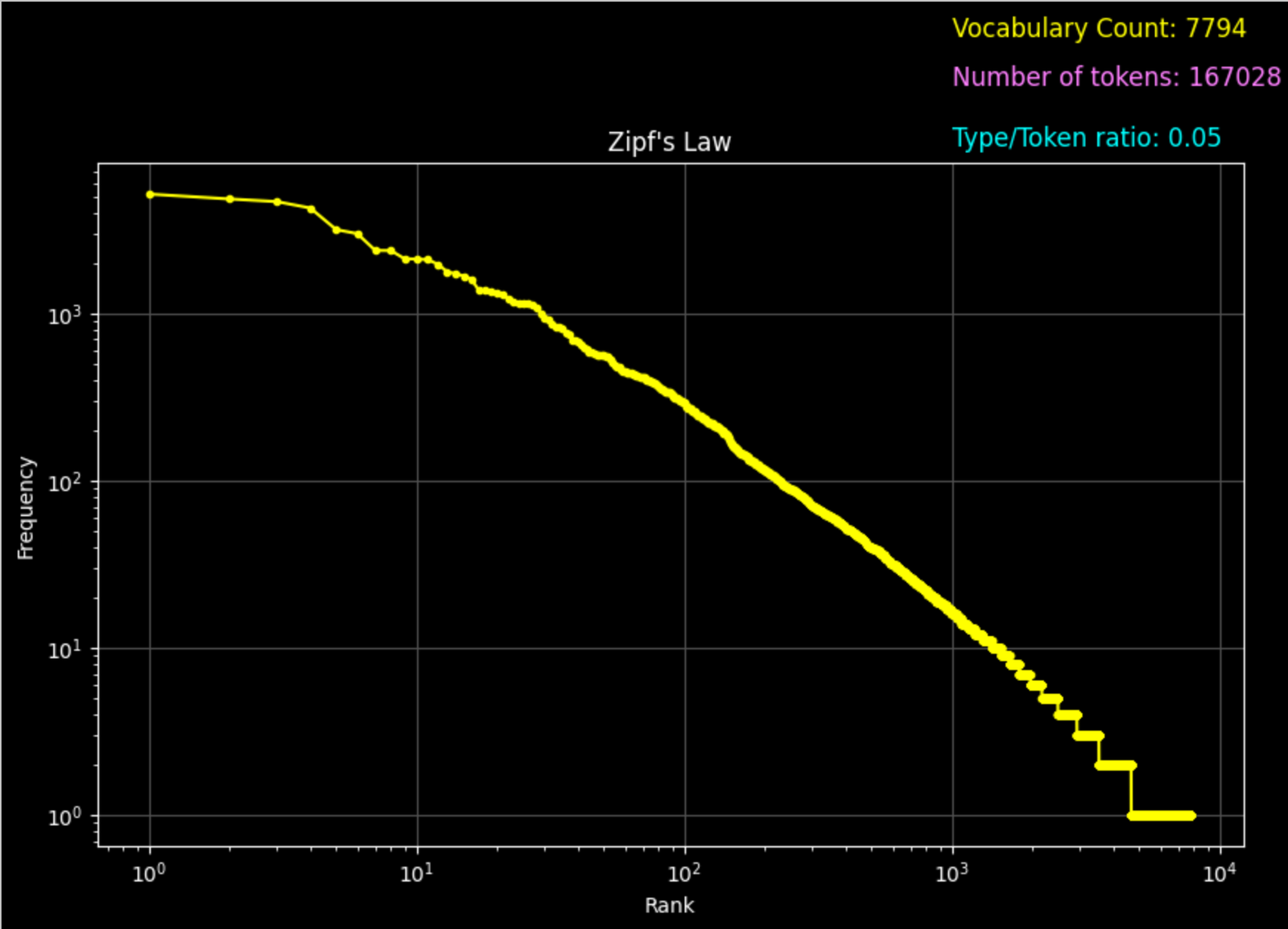
The line is not perfect. Its imperfections are informative.

At the very top, the few most frequent words sit slightly off the line. At the bottom, the singletons form discrete horizontal shelves, because a word can occur once or twice but never $1.4$ times.

Benoît Mandelbrot proposed a small correction that fits the head far better:

$$\begin{equation} f(r) \;\approx\; \frac{C}{(r + \beta)^{\alpha}}, \label{eq:mandelbrot} \quad\text{(3.3)} \end{equation}$$

where the shift $\beta$ flattens the curve for the first few ranks.

How large $\beta$ comes out depends almost entirely on how much of the tail you fit, because $\beta$ is what absorbs the bend. On Brown:

Fit the head alone and $\beta$ is exactly zero, so Mandelbrot buys nothing. Plain Zipf already describes the head. Fit every rank, which is what fit_mandelbrot does, and $\beta$ runs into the hundreds.

So a large $\beta$ is not a verdict on your corpus. It is what a single power law needs in order to cover a curve that bends. Note that $\alpha$ climbs with it, because both are absorbing the same curvature. Quote $\alpha$, $\beta$ and the rank range together, or none of them.

Why does language do this? Zipf’s own answer was a principle of least effort. Speakers want a small vocabulary of reusable words. Listeners want a large vocabulary of precise ones. The power law is where that tug of war settles.

Later work is a useful corrective. Surprisingly weak assumptions produce Zipf like curves, including random typing with a space bar. So the law’s existence tells us less than one might hope. Its consequences for us are concrete, and we return to them at the end of the chapter.

Fitting the exponent

Reading a law off a plot is not the same as measuring it. This section fits $\alpha$ properly, on data you can check by hand.

The corpus is a collection of Indian budget speeches, and the frequency table gives fifteen rows: ranks $1$ through $10$, and ranks $233$ through $237$. The top word, the, occurs $59{,}042$ times. The word at rank $10$ occurs $9{,}070$ times. The word at rank $235$ occurs $477$ times.

The first instinct is to solve for $\alpha$ from two points. Divide Equation (3.1) by itself at two ranks and the constant $C$ cancels:

$$\frac{f(1)}{f(10)} = \frac{C/1^{\alpha}}{C/10^{\alpha}} = 10^{\alpha}, \qquad\text{so}\qquad \alpha = \log_{10}\frac{f(1)}{f(10)} = \log_{10} 6.509 = 0.8136.$$

Now test that number where it was not fitted. Predicting rank $235$ gives $59{,}042 / 235^{0.8136} = 695$, against a measured $477$. The estimate is $46$ per cent too high.

The fix is to stop throwing data away. Take logarithms, and fit the line of Section 1.2.1 by least squares over all fifteen points:

$$\begin{equation} \hat{\alpha} \;=\; -\, \frac{\sum_i (x_i - \bar{x})(y_i - \bar{y})}{\sum_i (x_i - \bar{x})^2}, \qquad x_i = \log r_i, \quad y_i = \log f_i. \label{eq:zipf-ls} \quad\text{(3.4)} \end{equation}$$

That gives $\alpha = 0.9426$ and $C = 83{,}239$, and the same test now predicts $485$ against $477$. The error falls from $46$ per cent to under $2$.

These are exactly the values fit_zipf returns on the same fifteen rows, so the procedure above is the graded one, not an illustration of it.

Table 1.1 adds Mandelbrot’s correction to the comparison. The shift $\beta$ sits inside the logarithm, so least squares cannot reach it. Scan $\beta$, fit $\alpha$ and $C$ at each value, and keep the best. One extra parameter buys a third off the error.

Notice that the fitted $C = 83{,}239$ is larger than the observed $f(1) = 59{,}042$. The line does not pass through the top word, and it should not. The head is flatter than the body. A fit dominated by the head therefore understates $\alpha$, which is exactly what the two point estimate did.

Now the warning promised earlier. The Mandelbrot fit is a two parameter optimisation with a shallow valley:

Doubling $\beta$ moves $\alpha$ by more than three per cent and barely moves the error. Report $(\alpha, \beta)$ as a pair, or neither number means anything.

The exponent is not a constant

One more measurement settles what $\alpha$ actually is. Fit Brown over different rank ranges and the answer moves:

The tail falls faster than the head, so a wider window gives a steeper line. This is why the textbook claim $\alpha \approx 1$ is safe. It is a statement about the first few thousand ranks and nothing more.

An exponent quoted without its fitting range is not a measurement. Report the range every time.

Zipf as a probability

Equation (3.1) gives counts. Divide by the total count and it becomes a distribution over the vocabulary:

$$\begin{equation} p(r) \;=\; \frac{r^{-\alpha}}{H_{V,\alpha}}, \qquad H_{V,\alpha} \;=\; \sum_{k=1}^{V} k^{-\alpha}, \label{eq:zipf-prob} \quad\text{(3.5)} \end{equation}$$

where $H_{V,\alpha}$ is the generalised harmonic number. It is the normaliser that makes the probabilities sum to one, and it is what makes the next quantity computable.

Now $p(r)$ is the chance that a token drawn at random from the corpus is the rank $r$ word. Summing it gives the coverage of the top $k$ words:

$$\begin{equation} \operatorname{Coverage}(k) \;=\; \sum_{r=1}^{k} p(r) \;=\; \frac{H_{k,\alpha}}{H_{V,\alpha}}. \label{eq:coverage} \quad\text{(3.6)} \end{equation}$$

This is the single most useful number in the chapter, because it converts a curve into a budget.

Read column two against column four of Table 1.2. About two per cent of the vocabulary carries about $69$ per cent of the running text. Equivalently, discarding the rarest $77$ per cent of the types costs under eight per cent of the tokens.

The model tracks the measurement closely at the head and drifts at the tail, for the reason the previous section gave. One $\alpha$ cannot bend twice.

Three later decisions rest on this table. A stop list is short because the head is short. A truncated vocabulary loses many types and few tokens. A subword vocabulary of $32{,}000$ pieces spends its whole budget on the head, and Chapter 5 shows what it does with the rest.

One caveat worth keeping. When $\alpha \le 1$, the sum $H_{V,\alpha}$ grows without bound as $V$ grows. The tail never becomes negligible, however much text you add.

Heaps’ law: the vocabulary never closes

Zipf’s law describes a frozen corpus. Heaps’ law describes what happens as a corpus grows.

Let $N$ be the number of tokens read so far, and $V(N)$ the number of distinct types seen. Empirically,

$$\begin{equation} V(N) \;\approx\; K \, N^{b}, \label{eq:heaps} \quad\text{(3.7)} \end{equation}$$

with $K$ usually between 10 and 100, and the exponent $b$ usually quoted between $0.4$ and $0.6$ for English.

Quote the two together, because they are coupled. A fit that raises $b$ must lower $K$ to pass through the same data, so a large $b$ always arrives with a small $K$. Pin $b$ on Brown and watch the best $K$ move with it:

So “$K$ between 10 and 100 and $b$ between 0.4 and 0.6” is one statement about a curve, not two independent ones. Brown measures $K = 16.18$ and $b = 0.5764$ in Section 1.5.1, and Figure 1.2 shows a smaller and more homogeneous corpus at $b = 0.78$ with $K$ under two. That figure is right; small corpora really do fit that high.

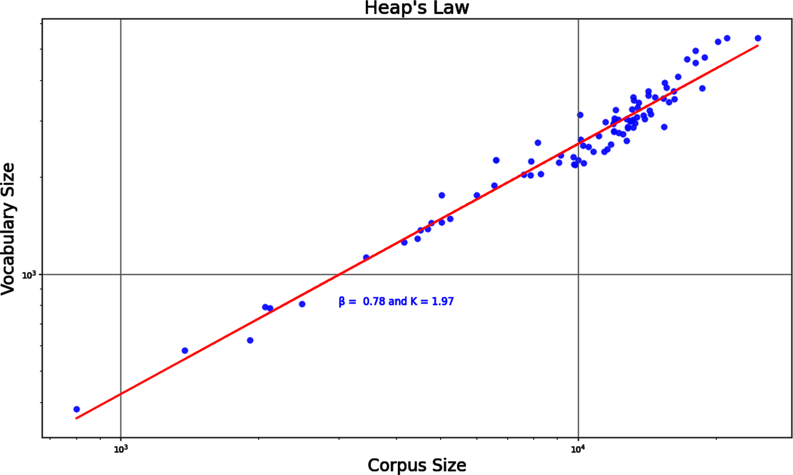
Two properties matter.

First, the exponent is less than one, so vocabulary growth decelerates. The second million tokens bring fewer new words than the first million did. Doubling a corpus does not come close to doubling its vocabulary.

Second, and this is the part with teeth, the function never flattens. There is no corpus size at which $V(N)$ stops growing, because a power law has no asymptote.

However much text you collect, the next document can still hold a word you have never seen. A name, a typo, a coinage, a chemical formula, a hashtag. The vocabulary of a natural language is not a closed set. Any system built around a fixed word list has already decided to fail on the tail.

You will check both properties in Project 1 by plotting $V(N)$ as your corpus streams past. In the spirit of Section 1.8 below, you will predict the curve’s shape before you draw it.

Fitting Heaps, and what extrapolation costs

Equation (3.7) linearises the same way Zipf’s law did:

$$\begin{equation} \log V(N) \;=\; \log K \;+\; b \log N. \label{eq:heaps-log} \quad\text{(3.8)} \end{equation}$$

So $b$ is a slope, and it is also an elasticity. Doubling the corpus multiplies the vocabulary by $2^{b}$. At $b = 0.5$, four times the text gives twice the vocabulary.

Sample the vocabulary every $1{,}000$ tokens, which is what fit_heaps does, and fit all $1{,}024$ points. Five of them:

The fit gives $b = 0.5764$ and $K = 16.18$. The corpus grew by a factor of a thousand. The vocabulary grew by a factor of $93$.

Fitting the full curve matters. Least squares on five hand-picked marks gives a visibly different pair, and it would not agree with the grader.

Now the experiment that matters more. Fit the law on the first $100{,}000$ tokens only, and use it to predict a corpus ten times larger. That prefix gives $b = 0.7176$ and $K = 3.50$, so

$$\hat{V}(10^{6}) = 3.50 \times (10^{6})^{0.7176} = 70{,}799, \qquad\text{against a measured } 43{,}648.$$

One decade of extrapolation, $62$ per cent too many types.

The cause is the same concavity that moved $\alpha$ earlier. The exponent $b$ is not a constant of the language either. It drifts downward as $N$ grows, because the log log curve bends gently. Fit over the range you will actually operate in, and treat any extrapolation as an upper bound.

That the error is an over-estimate is worth noticing. It is the safe direction for sizing an embedding table and the wrong direction for a cost estimate.

Zipf and Heaps are one fact seen twice

The two laws are not independent observations. If frequency falls as $r^{-\alpha}$, then a word at rank $r$ needs roughly $r^{\alpha}$ tokens of text before it appears at all. Reading that backwards, $N$ tokens reveal about $N^{1/\alpha}$ distinct types, so

$$\begin{equation} b \;\approx\; \frac{1}{\alpha}, \qquad \alpha > 1. \label{eq:zipf-heaps} \quad\text{(3.9)} \end{equation}$$

Brown fitted over all ranks gives $\alpha = 1.3492$, so Equation (3.9) predicts $b = 0.7412$. The measured $b$ is $0.5764$. The right order of magnitude, from two unrelated measurements, and not much better than that.

They do not agree exactly, and they should not. The derivation assumes a single $\alpha$ holds across the whole rank range, and Section 1.3 showed that it does not. The lesson is the relationship, not the decimal places. Steeper frequency decay means fewer rare words, which means slower vocabulary growth.

Type token ratio and the length trap

A natural summary of lexical richness is the type token ratio

$$\begin{equation} \operatorname{TTR} \;=\; \frac{V}{N}, \label{eq:ttr} \quad\text{(3.10)} \end{equation}$$

which is vocabulary size divided by text length. Rich, varied prose should score high. Repetitive, formulaic text should score low. And it does.

But there is a trap, and Heaps’ law describes it exactly. Since $V \approx K N^{b}$ with $b < 1$, we get $\operatorname{TTR} \approx K N^{\,b-1}$, which falls as $N$ grows.

Take a 1,000 word essay and a 100,000 word novel by one author. Their TTRs will differ wildly, and the novel’s will be far lower. There is no stylistic reason for it. TTR is not a property of a text. It is a property of a text at a length.

Brown’s own fit, $K = 16.18$ and $b = 0.5764$, puts numbers on that:

Same author, same style, four different answers. The measured column is the one that matters, and it falls by a factor of ten.

The first row is worth pausing on. The fitted law is good near a million tokens and poor at a thousand, because the log log curve is concave and $1{,}024$ points pull the line towards the large $N$ end. A fitted law is a summary of a curve, not an oracle for every point on it.

The trap, measured

Table 1.3 runs the experiment on six genres of Brown. The raw column uses the whole genre. The standardised column cuts each genre into non-overlapping windows of $8{,}000$ tokens, computes TTR in each, and averages them.

Raw TTR crowns humour as the richest genre in Brown. Humour is also the shortest genre in Brown, at $18{,}450$ tokens against $164{,}036$ for learned prose. The measurement is reading length, not style.

Two rankings actually reverse. Raw TTR puts fiction above press reportage; on equal windows press reportage wins. Raw TTR puts government above learned prose; on equal windows learned prose wins. Neither reversal is noise. Both hold at every window size from $2{,}000$ tokens to $18{,}000$.

The discipline that follows is simple and not negotiable. Never compare type token ratios across samples of different sizes. Compare equal length slices, or use a length corrected variant.

Length corrected variants

The measure used in Table 1.3 is the mean segmental type token ratio. Cut the text into $m$ windows of fixed size $W$ and average:

$$\begin{equation} \operatorname{MSTTR} \;=\; \frac{1}{m}\sum_{j=1}^{m} \frac{V_j}{W}. \label{eq:msttr} \quad\text{(3.11)} \end{equation}$$

It is simple and it works. Its weakness is that the answer still depends on $W$, so $W$ must be reported and held fixed across everything being compared.

A cheaper variant is the root type token ratio, $V/\sqrt{N}$. That is Equation (3.7) with $b$ forced to $0.5$. It only removes the length effect where $b$ really is near $0.5$. Brown’s is $0.58$, which is close enough to make it tempting and far enough to bias a comparison.

The honest summary of lexical richness is neither. It is the fitted pair $(K, b)$ from Section 1.5.1, which describes the whole curve rather than one point on it.

Project 1 asks you to compare your corpus against a contrast genre, and it fixes the sample size for exactly this reason. When the measured TTRs still differ, the difference is real. Legal boilerplate and technical templates repeat themselves. Fiction does not.

What the laws mean for everything downstream

These three regularities look like curiosities. They are the standing constraints under which every model in this book operates.

Which knob moves tokens, and which moves types

The laws also price the preprocessing decisions of Chapter 2. Measured on Brown, each figure a share of the raw counts:

Read the two columns against each other. Stop word removal takes $44$ per cent of the tokens and $0.2$ per cent of the types. That is Zipf’s law stated as an engineering fact. Stop words are very few types carrying very many tokens.

Stemming is the mirror image. Every token stays where it is, and $35$ per cent of the vocabulary collapses.

Dropping every type seen five times or fewer removes $72$ per cent of the vocabulary and costs $5.9$ per cent of the tokens. That is the trade Table 1.2 priced, and it is why a fixed subword vocabulary is less of a sacrifice than it looks.

One thing barely moves at all. The Heaps fit goes from $K = 16.18$, $b = 0.5764$ to $K = 17.33$, $b = 0.5958$ once stop words and numbers are gone. The curve is a property of the language, not of your cleaning.

Try it yourself. code/worked_examples/empirical_laws.py prints every fit and table in this chapter. python3 empirical_laws.py mandelbrot shows $\beta$ climbing from $0$ to $403$ as the fitting range widens. python3 empirical_laws.py heaps pins $b$ and watches $K$ move, then extrapolates a decade and misses by $62$ per cent.

Run it in ColabNotebookSource

The head motivates weighting. The most frequent words are overwhelmingly function words. Glue like the and of appears everywhere and so distinguishes nothing. Any similarity measure built on raw counts will be dominated by exactly the words that carry least content. That is the problem inverse document frequency solves in Chapter 4. At bottom, tf-idf is a machine for discounting the Zipfian head.

The tail motivates smoothing. Roughly half the vocabulary occurs once. The exact fraction depends on corpus size and rises as the corpus shrinks. Full Brown gives $39.5$ per cent, its news genre $49$ per cent and its science fiction $62$ per cent. At any of those figures, reliable statistics exist for almost no specific word. Events unseen in training are not rare accidents. They are the normal case. That is why the zero probability problem of Chapter 10 is not a corner case to patch. It is the central difficulty of statistical language modelling. Every model, up to the largest LLM, must reserve belief for the unseen.

Heaps’ law motivates subwords. If the vocabulary never closes, a word level system meets out of vocabulary items forever. Mapping them all to one <unk> symbol, as in Chapter 10, throws their identity away. The modern answer is to decompose rare words into pieces that are in a closed set. That is the next chapter, and it is best read as a direct engineering response to Equation (3.7).

The empirical discipline

This chapter closes with a habit rather than a law.

Every quantitative claim above is checkable in minutes on any corpus you can lay hands on. The slope near $-1$. The exponent near $0.5$. The falling TTR. This course will repeatedly ask you to predict the number before you measure it.

The point is not ritual. A prediction forces your mental model into the open, where the measurement can correct it. A measurement taken with no prediction slides past the mind and teaches nothing.

Calibration is knowing how far off your guesses tend to be. It is a trainable skill. It is also the difference between a practitioner who understands a system and one who merely operates it.

We start training it on word counts because word counts are cheap. By the end of the book you will be predicting perplexities, attention patterns and retrieval failures the same way.

Further reading.

, Human Behavior and the Principle of Least Effort, is still a strange and rewarding read. give the sober statistical treatment of both laws. is the modern reference for the mathematics of the tail.